Matrix (mathematics)

src: i.ytimg.com

In mathematics, a matrix (plural: matrix ) is a rectangle array of numbers, symbols, or expressions, row and column . For example, the dimensions of the matrix below are 2 Ã € "3 (read" two three "), since there are two rows and three columns:

${\ displaystyle {\ begin {bmatrix} 1 & amp; 9 & amp; -13 \\ 20 & amp; 5 & ​​amp; -6 \ end {bmatrix}}.} Â Â$

Individual items in the matrix m ÃÆ'â € n A , often denoted by a _{i , j} , where max i = m and max j = < i> n , called elements or entries . Provided they have the same size (each matrix has the same number of rows and the same number of columns as the other), two matrices can be added or subtracted element by element (see Conformable matrix). The rule for matrix multiplication, however, is that two matrices may be multiplied only when the number of columns in the first equals the number of rows in both (that is, the inner dimensions are the same, n for A _{m , n} ÃÆ'â € " B _{n , p} ). Each matrix can be multiplied element-wise by a scalar of related fields. The main application of the matrix is ​​to represent a linear transformation, namely the generalization of a linear function such as f ( x ) = 4 x . For example, the rotation of a vector in three-dimensional space is a linear transformation, which can be represented by a rotational matrix R : if v is a column vector (matrix with only one column) space, product Rv is a column vector that describes the position of that point after the rotation. The product of two transformation matrices is a matrix representing the composition of two transformations. Another application of the matrix is ​​the system solution of linear equations. If the matrix is ​​square, it is possible to infer some of its properties by calculating its determinants. For example, a square matrix has an inverse if and only if its determinant is not zero. Insight into the geometry of linear transformation can be obtained (together with other information) of the eigenvalues ​​of the matrix and eigenvectors.

Matrix applications are found in most scientific fields. In every branch of physics, including classical mechanics, optics, electromagnetism, quantum mechanics, and quantum electrodynamics, they are used to study physical phenomena, such as the movement of rigid bodies. In computer graphics, they are used to manipulate 3D models and project them onto 2-dimensional screens. In theory and probability statistics, the stochastic matrix is ​​used to describe the probability circuit; for example, they are used in PageRank algorithms that rank pages in Google search. The calculus matrix generalizes classical analytic notions such as derivatives and exponentials to higher dimensions. Matrices are used in economics to describe the system of economic relations.

The main branch of numerical analysis is devoted to the development of efficient algorithms for matrix calculations, centuries-old subjects and currently a growing research area. The matrix decomposition method simplifies calculations, both theoretically and practically. Algorithms that are matched with certain matrix structures, such as sparse matrices and near-diagonal matrices, speed up calculations in finite element methods and other calculations. The infinite matrix occurs in planetary theory and in atomic theory. A simple example of an infinite matrix is ​​a matrix representing a derived operator, acting on the Taylor series of a function.

Video Matrix (mathematics)

Definisi

A matrix is a rectangular array of numbers or other mathematical objects whose operations such as addition and multiplication are defined. Most commonly, the matrix above the F field is a scalar rectangle array each of which is a member of F . Most of this article focuses on the real and complex matrix , ie the matrix whose elements are real numbers or complex numbers, respectively. The more common types of entries are discussed below. For example, this is a real matrix:

${\ displaystyle \ mathbf {A} = {\ begin {bmatrix} -1.3 & amp; 0.6 \\ 20.4 & amp; 5.5 \\ 9.7 & amp; -6.2 \ end {bmatrix}}.}$

The numbers, symbols, or expressions in the matrix are called entries or elements . The horizontal and vertical entry lines in the matrix are called row and columns , respectively.

Size

The matrix size is determined by the number of rows and columns it contains. A matrix with m rows and n columns are called matrices m Ã, ÃÆ'â € " i> m -by- n matrix, while m and n are called the dimensions . For example, the matrix A above is a matrix of 3Ã,Ã Ã ¢ â, ¬ Ã, 2.

A matrix with one row is called row vector , and that has a single column called column vector . Matrices with the same number of rows and columns are called square matrices . Matrices with infinite number of rows or columns (or both) are called infinite matrices . In some contexts, such as computer algebra programs, it is important to consider a matrix with no rows or no columns, called empty matrices .

Maps Matrix (mathematics)

Notation

The specifications of the symbolic matrix notation vary widely, with some prevailing trends. The matrix is ​​typically denoted by capitalization (such as A in the example above), while the corresponding lowercase letters, with two subscript indexes (e.g., a ₁₁ , or a _1.1 ), represents the entry. In addition to using capital letters to symbolize matrices, many authors use a special typography style, generally bold (non-oblique), to distinguish matrices from other mathematical objects. The alternative notation involves the use of a double underline with the variable name, with or without bold style, (for example, ${\ displaystyle {\ underline {\ underline {A}}}}$ ).

The entries in the i -th and j -second column matrices A are sometimes referred to as i , j , ( i , j ), or ( i , j ) ^{a _ij . The alternative notation for the entry is A [ i, j ] or A _{i, j} . For example, the entry (1.3) of the following matrix A is 5 (also denoted by a _{13 1,3} , A [ 1,3 ] or A _{1, 3} ):}

${\ displaystyle \ mathbf {A} = {\ begin {bmatrix} 4 & amp; -7 & amp; \ color {red} {5} & amp; 0 \\ - 2 & amp; 0 & amp; 11 & amp; 8 \\ 19 & amp; 1 & amp; -3 & amp; 12 \ end {bmatrix}}} Â Â$

Kadang-kadang, entri dari matriks dapat didefinisikan oleh rumus seperti a _{i , j} = f ( i , j ). Sebagai contoh, masing-masing entri dari matriks berikut ini A ditentukan oleh a _ij = i - j .

${\ displaystyle \ mathbf {A} = {\ begin {bmatrix} 0 & amp; -1 & amp; -2 & amp; -3 \\ 1 & amp; 0 & amp; -1 & amp; -2 \\ 2 & amp; 1 & amp; 0 & amp; -1 \ end {bmatrix}}}  ÂÂ$

In this case, the matrix itself is sometimes defined by that formula, in square brackets or double brackets. For example, the matrix above is defined as A = [i> i - j ], or A = ((< i> i - j )). If the matrix size is m ÃÆ'â € " n , the formula mentioned above f ( i j ) apply to all i = 1,..., m and all j = 1,..., < i> n . This can be specified separately, or using m ÃÆ'â € " n as a subscript. For example, the matrix A above is 3 Ã € "4 and can be defined as A = [i> i - j = 1, 2, 3, j = 1,..., 4), or A = [ i - j ] _{3 ÃÆ'â € "4} .

Some programming languages ​​use multiple array subscripted (or array arrays) to represent the matrix m -ÃÆ' â € "- n . Some programming languages ​​start array array indexing at zero, in this case the entries of the m -by- n matrix are indexed by 0 <= i <= m - 1 and 0 <= j <= n - 1 . This article follows a more general convention in the writing of mathematics in which enumeration starts from 1.

The asterisks are sometimes used to refer to the whole row or column in the matrix. For example, a _{i , *} refers to the line i ^th from A , and a _{*, j} refer to column j ^th from A . The set of all matrices m -by- n is denoted by M ( m , n ).

src: i.stack.imgur.com

Basic operation

There are a number of basic operations that can be applied to modify matrices, called matrix additions, scalar doubling , transpositions , matrix multiplication >, line operations , and submatrix .

Additionally, scalar multiplication and transposition

The usual number properties are extended to the operation of this matrix: for example, the addition is commutative, that is, the number of matrices does not depend on summary order: A Ã, B Ã, = < B> B Ã, A . This transpose is compatible with additional summaries and scalars, as disclosed by ( c A ) ^T = < b> A ^T ) and ( A Ã, B A ^T Ã, B ^T . Finally, ( A ^T ) ^T Ã, = Ã, A .

Multiplication matrix

multiplication of two matrices is determined if and only if the number of columns from the left matrix equals the right number of matrix rows. If A is the matrix m -by- n and B is n -by - p matrix, the matrix product AB the matrix whose entries are supplied by the point product from the corresponding row of A and corresponding columns from B : $Â\; ÂÂ\; Â\; Â\; ÂÂ\; Â\; Â\; Â\; Â{\displaystyle Â\; Â\; Â\; Â\; Â\; Â\; Â\; Â[Â\; Â\; Â\; Â\; Â\; Â\; Â\; ÂÂ\; Â\; Â\; Â\; Â\; Â\; Â\; Â\; Â\; Â\mathbf{A}Â\; Â\; Â\; Â\; Â\; Â\; Â\; Â\; Â\; Â\mathbf{B}Â\; Â\; Â\; Â\; Â\; Â\; Â\; ÂÂ\; Â\; Â\; Â\; Â\; Â\; Â\; Â{]}_{Â\; Â\; Â\; Â\; Â\; Â\; Â\; Â\; Â\; Â\; Â\; Â\mathrm{me}}}$,             j                           =                   A                      me ,             1                                     B                      1 ,             j                                             A                      me ,             2                                     B                      2 ,             j                                   ?                           A                      me ,             n                                     B                      n ,             j                           =                  ?                      r =             1                                n                                     A                      me ,             r                                     B                      r ,             j                             Annotation encoding = "application/x-tex"> {\ displaystyle [\ mathbf {AB}] _ {i, j} = A_ {i, 1} B_ {1, j} A_ {i, 2 } B_ {i, n} B_ {n, j} = \ sum _ {r = 1} ^ {n} A_ {i, r} B_ {r, j}}   ,

The matrix multiplication meets the rules ( AB ) C = A ( BC ) (associativity), and ( A B ) C = AC BC and C (< b> A B ) = CA CB (left and right distributions), whenever the size of the matrix is ​​such that various products defined. The AB product can be defined without BA specified, ie if A and B are m -by- n and n -by- k the matrices, respectively, and m ? k . Even if both products are defined, they need not be the same, that is, generally

AB ? BA ,

that is, the non-commutative multiplication matrix, in contrast with the (rational, real, or complex) number whose product does not depend on the order of the factor. Examples of two non-commuter matrices to each other are:

${\ displaystyle {\ begin {bmatrix} 1 & amp; 2 \\ 3 & amp; 4 \\\ end {bmatrix}} {\ begin {bmatrix} 0 & amp; 1 \\ 0 & amp; 0 \\\ end {bmatrix}} = {\ begin {bmatrix} 0 & amp; 1 \\ 0 & amp; 3 \\\ end {bmatrix}},} Â Â$

sedangkan

${\ displaystyle {\ begin {bmatrix} 0 & amp; 1 \\ 0 & amp; 0 \\\ end {bmatrix}} {\ begin {bmatrix} 1 & amp; 2 \\ 3 & amp; 4 \\\ end {bmatrix}} = {\ begin {bmatrix} 3 & amp; 4 \\ 0 & amp; 0 \\\ end {bmatrix}}.}  ÂÂ$

In addition to the usual matrix multiplication just described, there are other operations that are less commonly used in matrices that can be considered as multiplication forms, such as Hadamard products and Kronecker products. They appear in solving equations of matrices like Sylvester's equations.

Line operations

There are three types of line operations:

1. an additional line, which is adding a line to another line.
2. row multiplication, ie multiplying all entries from a row with non-zero constants;
3. the switching line, which exchanged two matrix rows;

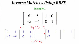
This operation is used in several ways, including solving linear equations and finding the inverse matrix.

Submatrix

Sebuah submatrix dari matriks diperoleh dengan menghapus setiap kumpulan baris dan/atau kolom. Sebagai contoh, dari matriks 3-oleh-4 berikut, kita dapat menyusun submatrix 2-oleh-3 dengan menghapus baris 3 dan kolom 2:

${\ displaystyle \ mathbf {A} = {\ begin {bmatrix} 1 & amp; \ color {red} {2} & amp; 3 & amp; 4 \\ 5 & amp; \ color {red } {6} & amp; 7 & amp; 8 \\ warna {red} {9} & amp; \ color {red} {10} & amp; \ color {red} {11} & amp; \ color {red} {12} \ akhiri {bmatrix}} \ rightarrow {\ begin {bmatrix} 1 & amp; 3 & amp; 4 \\ 5 & amp; 7 & amp; 8 \ end {bmatrix}}.}  ÂÂ$

Minors and cofactors of the matrix are found by calculating the determinants of certain submatrices.

the main submatrix is the square submatrix obtained by deleting certain rows and columns. Definitions vary from author to author. According to some authors, the main submatrix is ​​the submatrix in which the row index sets remain the same as the remaining set of index columns. Other authors define the main submatrix as the first k row and column, for some numbers k , which are fixed; this submatrix type has also been called the leading main submatrix .

src: i.ytimg.com

Linear equations

The matrix can be used to write and work compactly with some linear equations, the system of linear equations. For example, if A is a matrix of m -by- n , x denotes a column vector (i.e. n ÃÆ'â € "1-matrix) of n the variables x ₁ sub> 2 ,..., x _n , and b ÃÆ' â € "1-column vector, then the matrix equation

${\ displaystyle \ mathbf {Ax} = \ mathbf {b}}$

setara dengan sistem persamaan linear

${\ displaystyle A_ {1,1} x_ {1} A_ {1,2} x_ {2} \ cdots A_ {1, n} x_ {n} = b_ {1}}  ÂÂ$

${\ displaystyle \ vdots}  ÂÂ$

${\ displaystyle A_ {m, 1} x_ {1} A_ {m, 2} x_ {2} \ cdots A_ {m, n} x_ {n} = b_ {m}}  ÂÂ$

Using a matrix, this can be solved more compact than it is possible by writing all the equations separately. If n = m and its equations are independent, this can be done by writing

$Â\; ÂÂ\; Â\; Â\; ÂÂ\; Â\; Â\; Â\; Â{\displaystyle Â\; Â\; Â\; Â\; Â\; Â\; Â\; ÂÂ\; Â\; Â\; Â\; Â\; Â\; Â\; Â\; Â\; Â\mathbf{x}Â\; Â\; Â\; Â\; Â\; Â\; Â\; ÂÂ\; Â\; Â\; Â\; Â\; Â\; Â\; Â=Â\; Â\; Â\; Â\; Â\; Â\; Â\; Â{Â\; Â\; Â\; Â\; Â\; Â\; Â\; Â\; Â\; Â\; Â\; Â\mathbf{A}Â\; Â\; Â\; Â\; Â\; Â\; Â\; Â\; Â\; Â}^{Â\; Â\; Â\; Â\; Â\; Â\; Â\; Â\; Â\; Â\; Â\; Â-Â\; Â\; Â\; Â\; Â\; Â\; Â\; Â\; Â\; Â\; Â\; Â1Â\; Â\; Â\; Â\; Â\; Â\; Â\; Â\; Â\; Â}Â\; Â\; Â\; Â\; Â\; Â\; Â\; ÂÂ\; Â\; Â\; Â\; Â\; Â\; Â\; Â\; Â\; Â\mathbf{b}Â\; Â\; Â\; Â\; Â\; Â\; Â\; ÂÂ\; Â\; Â\; Â\; Â\; Â}Â\; Â\; Â\; ÂAnnotation\; encoding\; =\; "application/x-tex">\; \{\backslash \; displaystyle\; \backslash \; mathbf\; \{x\}\; =\; \backslash \; mathbf\; \{A\}\; ^\; \{-\; 1\}\; \backslash \; mathbf\; \{b\}\}\; Â\; Â$

where A ^-1 is the inverse matrix of A . If A has no inverse, the solution if present can be found using a common inverse.

src: i.stack.imgur.com

Linear transformation

The matrix and matrix multiplication reveal their essential features when it relates to the linear transforms , also known as the linear map . A produces a linear transformation R ^{> n} -> R ^m maps each x R ⁿ to a product (matrix) Ax sup> m . Instead, each linear transformation f : R ^{n m} appears from the unique matrix m -by- n A : explicitly, j ) - entry of A is i ^th j ), where e < sub> j = (0,..., 0,1,0,..., 0) is the unit vector with 1 at i> ^th and 0 elsewhere. The matrix A is said to represent the linear map f , and A is called the transform matrix .

Misalnya, matriks 2ÃÆ' — 2

Source of the article : Wikipedia